Polynomial Curve Fitting

Polynomial Curve Fitting is an example of Regression, a supervised machine learning algorithm.

End Goal of Curve Fitting

We observe a real-valued input variable, 𝑥 , and we intend to predict the target variable, 𝑡 . Polynomial Curve fitting is a generalized term; curve fitting with various input variables, 𝑥 , 𝑦 , and many more.

We will see curve fitting on a synthetic dataset.

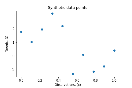
For the synthetic dataset, we will generate the data points from a function sin2𝜋𝑥 with some random normal noise included.

## Imports
import warnings
import numpy as np
import matplotlib.pyplot as plt

## Set a seed
np.random.seed(0)

## Create Synthetic Dataset
x = np.linspace(0.0, 1.0, num=10)
t = (np.sin(2*np.pi*x)) + np.random.normal(0, 1, 10)

txt="Fig 1.1: Scatter plot of the observations with targets"
plt.scatter(x, t)
plt.xlabel("Observations, (x)")
plt.ylabel("Targets, (t)")
plt.title("Synthetic data points")
plt.show()

Figure 1.1

In mathematical Notations

The scatter plot in Figure 1.1 possesses an underlying regularity which we want to learn. This is an intricate problem since we have a finite number of data set with noises embedded.

Now, let’s consider a simple approach for curve fitting. Consider a polyomial function of the form:

where,

M = order of the polynomial

𝑤0,𝑤1,…,𝑤𝑀 = polynomial coefficients (denoted by vector, v )

Remember: 𝑦(𝑥,𝑤) is non linear function of 𝑥 but the linear function of coefficients, 𝑤 . Functions which are linear in terms of unknown parameters are called linear models.

Determinine the unknown parameters, w

The value of the coefficients is found by fitting the polynomial to the training dataset. For this, we minimize the error function that calculates the misfit between function 𝑦(𝑥,𝑤) and the training data points. One of the widely used error functions is the Sum of the Squares of the Errors (SSE).

1/2 has a convenience, which we will see in later chapters. SSE is a non-negative quantity and we wish to choose unknown parameters, w to make SSE minimum. The error function is quadratic so its first derivative for coefficients, w will be a linear equation with w as unknown. So, we can solve for the unique values of w, which we will denote by w∗ since this set of parameters minimize the error function’s value and the resulting curve is given by 𝑦(𝑥,𝑤∗).

Determine the order of the polynomial, M

Now, we need to find M for the curve. M is the order of the polynomial and selection of the order of the polynomial comes under a broad topic, Model Comparison or Model Selection.

• With M=0

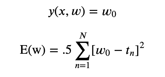
For the elucidation, we will see how the unique value for w is found out with M=0 , since it is easiest among all possible valued of M to calculate manually. For M=0 , the coefficient(unknown parameter) is denoted by 𝑤0 , so we wil find 𝑤0 now.

The Error function fully expanded seems like:

from sympy import *
w_0 = Symbol('w_0')
E = .5 * ((w_0 - 1.76405235)**2 + (w_0 - 1.04294482)**2+ (w_0 - 1.96354574)**2+ (w_0 - 3.1069186)**2+ 
        (w_0 - 2.20957813)**2+ (w_0 + 1.31929802)**2+ (w_0 - 0.08406301)**2+ (w_0 + 1.13616496)**2+ 
        (w_0 + 0.74600646)**2+ (w_0 - 0.4105985)**2) 

Now, we compute the first derivative of E(𝑤0) with respect to 𝑤0 and solve it for 𝑤0 . Mathematically:

In case, we choose higher M , we would have more more unknown parameters, to state there would be M+1 , unknown parameters and we would find all the unknown parameters by simply taking the partial derivative of the error function w.r.t to all the unknown parameters.

## Calculate the partial derivative w.r.t w_0
Eprime = E.diff(w_0)

## See the output
print(Eprime)

Output: 10.0*w_0 - 7.38023171

## Solve the linear equation of Eprime by equating to 0.
w_0 = solve(Eprime)
print(w_0)

Output: [0.738023171000000]

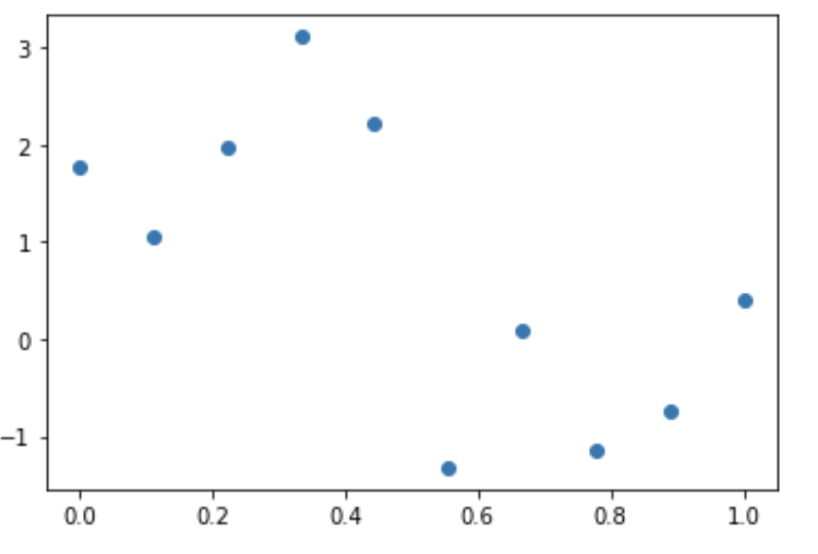
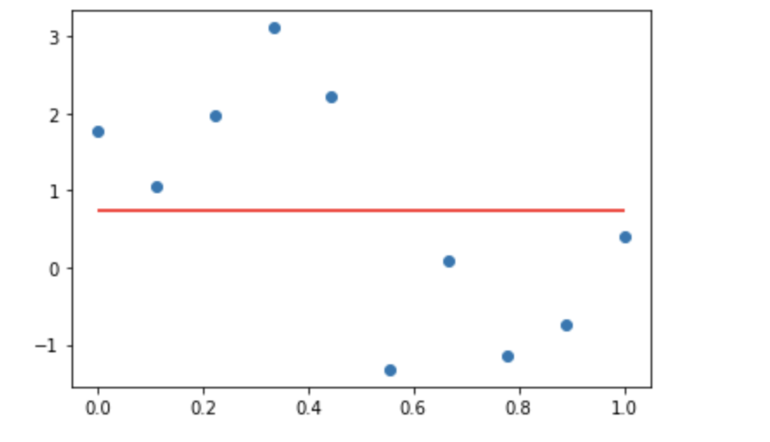
So, now this is the value for 𝑤0 to minimize the error function. Let’s plot this line on the original data points set.

𝑦=0.739

plt.scatter(x, t)
plt.show()

fig, ax = plt.subplots()
ax.scatter(x, t)
ax.hlines(y=0.739, xmin=0, xmax=1,color='r')
plt.show()

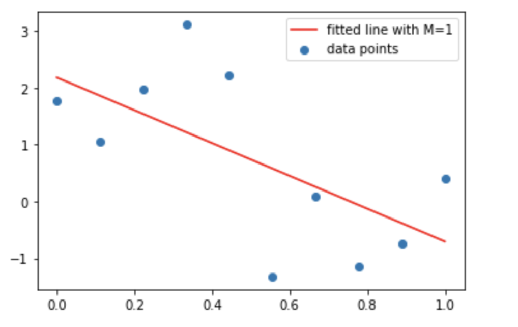
Similarly, now we will see the coefficient for other valued of M . We will see for M=1,3,9 . For the coefficient calculation, we won’t go step by step as we did for M=0 . We will use a numpy librbay, numpy.polyfit which performs the least squares polynomial fit with the number of order specified.

## For M =1
coefs = np.polyfit(x, t, 1)
print(coefs)

Output: [-2.87998582 2.17801608]

Now, we will plot the curve with these coefficients.

## Fitted Curve
y = coefs[1] + coefs[0]*x 

## Plot the fitted curve
plt.scatter(x, t, label = 'data points')
plt.plot(x, y, c ='r', label ='fitted line with M=1')
plt.legend()
plt.show()

## For M = 3
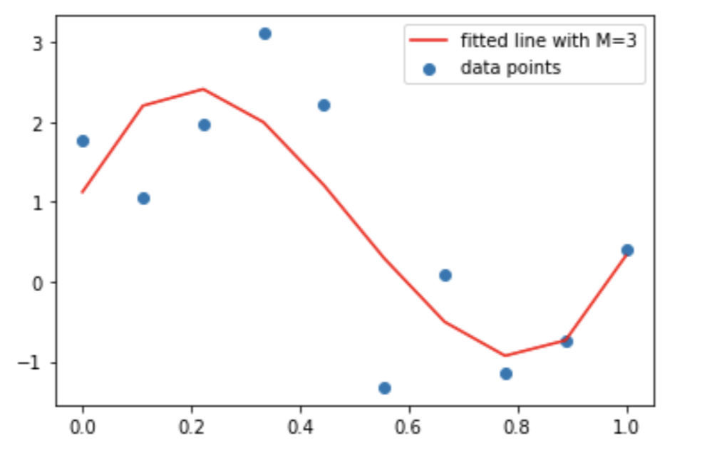
coefs = np.polyfit(x, t, 3)
print(coefs)

Output: [ 30.12650107 -45.28783042 14.36416336 1.12207597]

## Fitted Curve
y = coefs[3] + coefs[2]*x + coefs[1]*x**2 + coefs[0]*x**3

## Plot the fitted curve
plt.scatter(x, t, label = 'data points')
plt.plot(x, y, c ='r', label ='fitted line with M=3')
plt.legend()
plt.show()

## For M = 9
coefs = np.polyfit(x, t, 9)
print(coefs)

Output: [-3.07007894e+05 1.34937867e+06 -2.47898606e+06 2.47025924e+06 -1.44948523e+06 5.08745738e+05 -1.03533067e+05 1.11036868e+04 -4.76434849e+02 1.76405235e+00]

 ## Fitted Curve
y = coefs[9] + coefs[8]*x + coefs[7]*x**2 + coefs[6]*x**3 + coefs[5]*x**4 + coefs[4]*x**5 + coefs[3]*x**6 + coefs[2]*x**7 + coefs[1]*x**8 + coefs[0]*x**9

## Plot the fitted curve
plt.scatter(x, t, label = 'data points')
plt.plot(x, y, c ='r', label ='fitted line with M=9')
plt.legend()
plt.show()

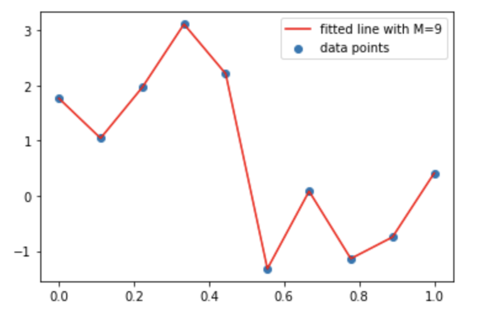
Conclusions/Inferences Now, from the above plots and orders of the polynomial, things are clear to an extent. We see that the order, M=0 and M=1 fit poorly to the data points. When we opted for the much higher order, i.e., 9 then, the data points are completely captured by the fitted curve. In this case, the error is 0 since the fitted curve passes through each training data point and there are no residuals(errors). However, this fitted curve oscillates heavily and poorly represents the underlying function, sin2𝜋𝑥 . This behavior is widely popular as Over-fitting.

The polynomial with the third-order seems to mimic the sin2𝜋𝑥 most decently, thus making this the best fit.

As stated earlier, the main aim of the Polynomial Curve Fitting is to achieve the best fit that generalizes the most. Generalization is the ability to categorize correctly new examples that differ from those used in the training dataset. And the polynomial with order 9 is very well on the training dataset but it fails in generalizing to the new data points. Hence, we called this fit an over-fit. The polynomial curve should be able to incorporate the new unseen data points too. Therefore, we have a training set and testing set, where the testing set is used to assess the fitted polynomial.

Over-fitting is fatal to the models. Hence, we must try to get rid of this. We can do so by:

• Increasing the number of data points while training.
• Using regularization parameters. (not covered here)