Probability Densities

Probability Distributions

Probability distribution for a random variable is a function whose output is the probability of the outcomes of an experiment. In other words, it is a statistical function that provides us with all the outcomes of a random variable within a range in an experiment along with their probabilities of occurrence. The range is bounded by the minimum and maximum possible value that random variable can take.

Probability distributions can be classified into various types, such as Uniform Distribution, Normal Distribution, Poisson Distribution, Binomial Distribution, Bernoulli Distribution, etc.

Probability Distribution are primarily classified as:

• Discrete Probability Distribution
• Continuous Probability Distributions

Discrete Distribution->Probability Mass Function

Discrete Probability distribution deals with the discrete random variables. Discrete random variables take any value within discrete set of values. For example: The outcome of an experiment of rolling a die is an example of discrete random variable, since the possible outcomes are discrete and falls into the set {1, 2, 3, 4, 5, 6}. In this case, if we have a fair die, the probability of getting each of the outcomes is 16 , and the probability distribution function or in this case probability mass function would look like:

import matplotlib.pyplot as plt
outcomes = [1,2,3,4,5,6]
probabilities = [1/6, 1/6, 1/6, 1/6, 1/6, 1/6]
plt.bar(outcomes, probabilities)
plt.title("Probability Mass Function [Rolling a Fair Die]")
plt.ylabel("Probabilities")
plt.xlabel("Outcomes")
plt.show()

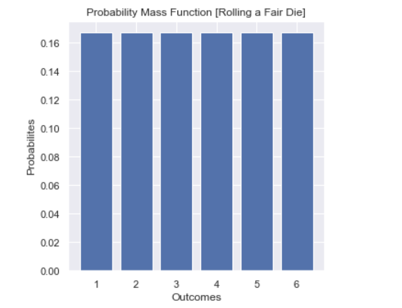
From the figure, we conclude that:

𝑃(1)=1/6

𝑃(2)=1/6

𝑃(3)=1/6

𝑃(4)=1/6

𝑃(5)=1/6

𝑃(6)=1/6

Continuous Distribution

Probability Density Function

Now, we are into continuous random variables, which take on any value from continuum, any real number. Hence, in this continuous probability distribution, commonly known as probability density function, the function doesn’t provide the probability for a single number or value as in the case of probability mass function. In this case, we have to take the range and see the probability for that range. The probability that any random variable takes on a particular value is 0 .

For example: Let’s define our continuous random variable as the weight of the students in the class. The weight of students in the class can not be measured accurately and thus exact weight of no individual is determinable. One randomly selected student might weight 137.56 pounds while another might weight 138.009 pounds. In this case, we are not able to exactly find the correct weight of each of the individuals and are rounding of or taking an approximation. Thus , finding the probability for a exact weight, i.e., 𝑃(𝑊𝑒𝑖𝑔ℎ𝑡=137) is not going to work. Instead, we will need to define an interval, such as 𝑃(136<𝑊𝑒𝑖𝑔ℎ𝑡<137) and probability distribution function will help us do this.

Let’s see the modeling of probability density function with small implementation.

import numpy as np
import matplotlib.pyplot as plt

mu, sigma = 136.5, 2 # mean and standard deviation
s = np.random.normal(mu, sigma, 1000) ## Random Normal Distribution Number Generator

plt.plot(bins, 1/(sigma * np.sqrt(2 * np.pi)) *
               np.exp( - (bins - mu)**2 / (2 * sigma**2) ),
          label = "Probability Density Function, p(x)")
plt.legend()
plt.xlabel("Weights")
plt.ylabel("Probabilities")
plt.title("Probability Density Function [Weights of the Students in a class]")
plt.show()

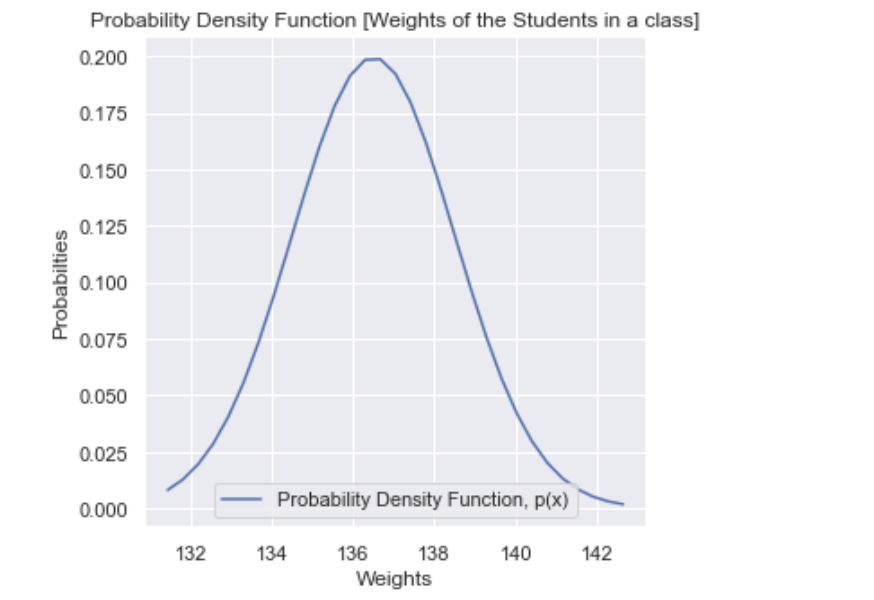
From the above probability density function graph, we can conclude the following points:

• Probabilities are non-negative, i.e., 𝑝(𝑥)>=0
• Probability of the random variable within an interval, (𝑎,𝑏) is given by:

• The sum of all the probabilities is 1 .

Note: The sum rule and product rules of probability is applicable to the case of probability densities. If 𝑥 and 𝑦 are two real variables, we can write sum and product rules as: