Understanding Linear Regression [1/3]

In the pool of machine learning algorithms, linear regression is the most often seen, used, and go-to supervised linear model. When I say this, what do I mean by linear model?

Linear models are the most basic, which explains their widespread use and appeal. If I were to sum up linear models in a single sentence, it would be a model in which features are combined linearly to produce an output.

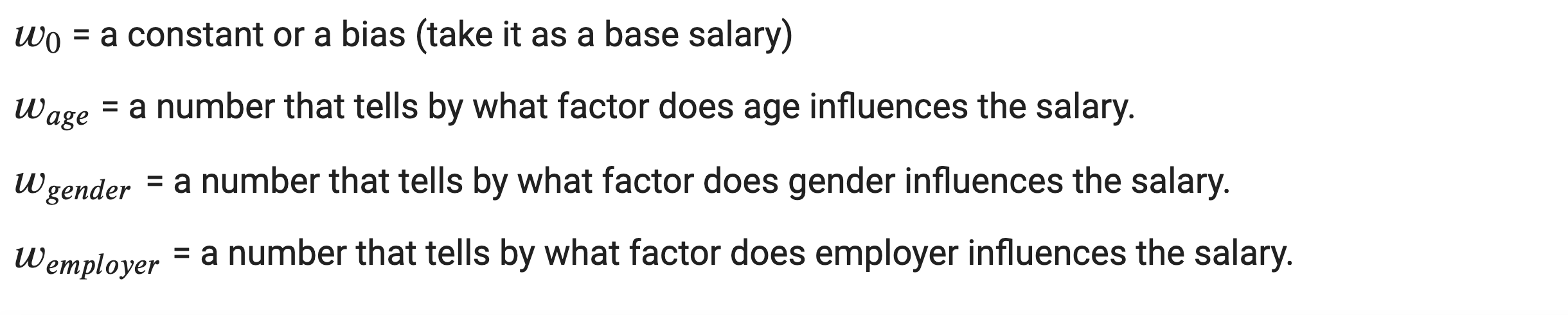
For instance, suppose we wish to create a linear model that predicts a salary of an individual. In this case, let’s take age of an individual, gender of an individual, and an employer as the inputs or features. The linear model would look like:

Now that we are warmed up, we will proceed towards building a strong understanding of the underlying mathematical concepts of linear regression. I assume, we are familiar with the basic knowledge on what linear regression is about. If not, here is the basic revisit of linear regression.

Data

Input: 𝑥 (i.e, measurements, covariates, features, independent variables)

Output: 𝑦 (i.e., response, dependent variable)

Goal

You need to find a regression function 𝑦 ≈ 𝑓(𝑥,𝛽) , where 𝛽 is the parameter to be estimated from observations.

For Simple Linear regression:

For Multiple Linear regression:

A regression method is linear if the prediction 𝑓 is a linear function of the unknown parameters 𝛽.

Linear regression finds several applications in our day to day life. Suppose, in a sales company; you need to maximize the sales; it is essential to know the weightage of each factor, such as advertisement, investment, recruitment to the sales. This is where you use linear regression. As such, we have numerous applications of linear regression.

While modeling linear regression, the standard estimation techniques make several assumptions about the predictor variables or input variables, response variable or output variable, and their relationship.

Some Assumptions of Linear Regression

1. Linear regression should be linear in parameters.

The response variable, 𝑦 is the function of input variables, 𝑥’s and parameters, 𝛽’s. But the linearity condition is up to parameters. The output variable should be linear in terms of parameters, not necessarily in terms of input variables.

For example: The equation below is linear in terms of both inputs and parameters, so hold the assumption.

Similarly, equation below is not linear in terms of inputs but linear in terms of parmaeters so it holds the assumption.

Lastly, the equation below is linear in terms of input but is not linear in terms of parameters, so it violates the assumption and is not a linear regression model.

1. Error or residuals should have constant variance and no autocorrelation.

An essential assumption of the linear regression model is that the residuals or errors have the same variance for all data points. This is called the homoscedasticity. If this variance is not constant (i.e. dependent on input variables, 𝑥′ s), then the linear regression model has heteroscedastic errors and this condition of heteroscedasticity might result incorrect parameters.

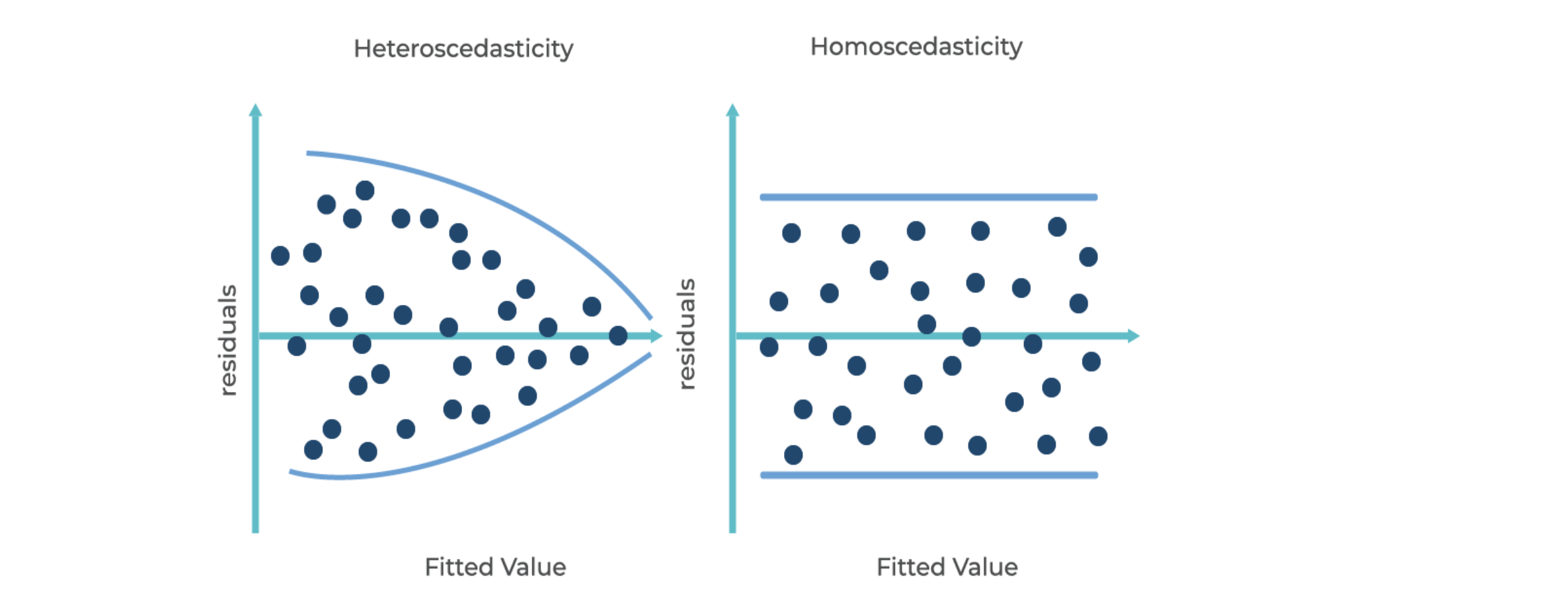
Above Figure shows the Homoscedasticity and Heteroscedasticity. The variance of errors is constant in homoscedasticity, while it’s not the case if errors are heteroscedastic. We always assume the errors to be homoscedastic.

Similarly, the assumption of no autocorrelation says that the error terms of different observations should not be correlated. In other words, errors or residuals should be IID (Independent and Identically Distributed).

Usually, in time-series data, we are likely to suffer from autocorrelation because each data in the next instant depends upon the data at the previous instant. So, error terms are somehow correlated.

1. There shouldn’t be multicollinearity.

Multi colinearity here means perfect colinearity. This assumption is for input variables. In simple linear regression, where we have a single input variable, this assumption doesn’t play any role, but in case of multiple linear regression, we should be careful. Any two or more sets of input variables should not be perfectly correlated. Perfect correlation might not make the predictor’s matrix full rank, which creates a problem in estimating the parameters.

For example, while predicting the house price, you can have many input variables, length, breadth, area, location, and many more. In this case, if you include the feature, area along with length, breadth, you might violate the assumptions because:

In such a situation, it is better to drop one of the three input variables from the linear regression model.

1. There should be a random sampling of observations.

The observations for the linear regression should be randomly sampled from any population. Suppose, you are trying to build a regression model to know the factors that affect the price of the house, then you must select houses randomly from a locality, rather than adopting a convenient sampling procedure. Also, the number of observations should always be higher than the number of parameters to be estimated.

Parameter Estimation Techniques

Now that you know the assumptions of Linear Regression, it’s time you know the techniques to find the parameters, i.e., intercept and regression coefficients. Earlier, we used Scikit-Learn’s LinearRegression predictor object to estimate 𝛽’s. It provides us with the optimized 𝛽’s. But now you should know how the optimized parameters are being calculated. There are different techniques by which you can find the parameters. Two of them are as follows:

• Least Squares Estimation

  In practice, observed data or input-output pair is given, and 𝛽’s are unknown. We use the given input-output pair to estimate the coefficients. The estimated intercept and regression coefficient later helps us in predicting the output value with the input values. There is an error or residual since the estimated regression can not satisfy all the output data points. Hence, we have an error or residual, which is the difference between the estimated output value and the actual output value. Errors can either be positive or negative. We can sum the errors to evaluate the estimated linear regression line. To get rid of the cancellation of the positive and negative error, we square the error and add then which is popularly called as Sum of Squares of errors or Residual Sum of Squares.

  This parameter estimation technique finds the parameters by minimizing the sum of squares. You will learn details on this technique with the mathematical formulation in the upcoming chapter. There are mainly three types of Least Squares:

  • Ordinary Least Squares

  • Weighted Least Squares

  • Generalized Least Squares

• Maximum Likelihood Estimation

Maximum likelihood estimation is a well known probabilistic framework for finding parameters that best describe the observed data. You find the parameters by maximizing the conditional probability of observing the data, 𝑥 given specific probability distribution and its parameters 𝛽’s. Detailed discussion on this technique is out of the scope.