Understanding Linear Regression [2/3]
Ordinary Least Squares with Simple Linear Regression
Since you have already been introduced to simple linear regression, we won’t discuss the details here.
The simple linear regression model is:

where, we need to estimate the parameters, intercept(𝛽0) and slope(𝛽1).
Let’s recall an Advertising dataset and simple linear regression performed on scatter plot of sales Vs. TV. With the help of Scikit-Learn, we were able to fit the best regression line among all the possibilities. Here is a snapshot:
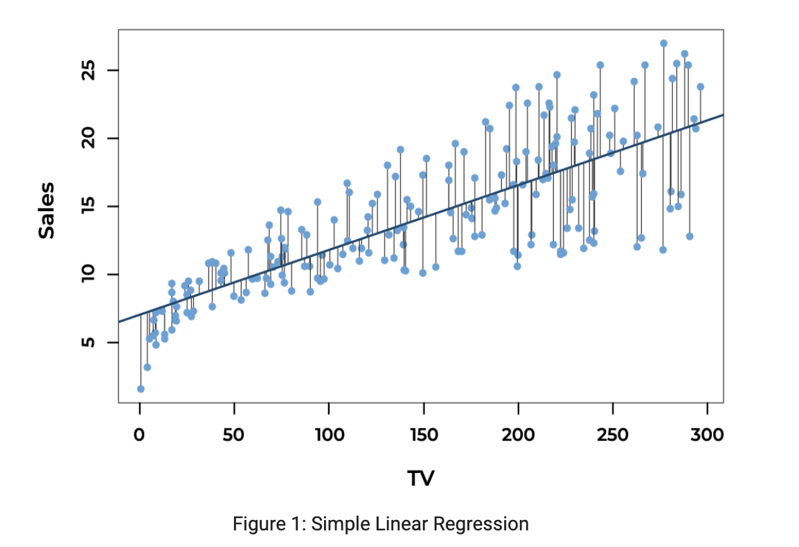
The blue line is a simple linear regression line with output 𝐲 as sales and 𝐱 as TV. The residual or error, 𝜖 is the difference between the observed value, y𝑖, and predicted value, yhat . The observed value is the actual output data point, which is all red dots in the figure, and the predicted value is the point given by the blue regression line. Error for each output data point is shown by the vertical distance from the actual output data point to the predicted point on a regression line.
The predicted output value is:

The observed (actual) output value is:

Where 𝜖𝑖 is a random error, not a parameter. The error 𝜖𝑖 as (y-yhat) can either be positive or negative or even 0 sometimes. As we can see in the figure, vertical lines are on either side of the regression line. To avoid the cancellation of the error while summing errors, we square each error and sum them, called Residual Sum of Squares (RSS) or Sum of Squared Errors (SSE).

The summation is indexed from 1 to 𝑛, since we have 𝑛 samples. Sum of Squared Errors (SSE) is the function of 𝛽0 and 𝛽1 . We can also take it as Loss function. The main principle of Least Squares is that we should end up choosing intercept (𝛽0) and slope (𝛽1) such that the overall sum is minimum.
Thus, to estimate the parameters, we minimize the sum of squared error. Sum of Squared Errors (SSE) can also be written as:

yhat is replaced with the simple linear regression model equation. Since we tend to minimize SSE , it is also called an objective function. Since the objective function, SSE is a squared term, it is always positive. If we plot objective function, it would be a convex graph facing upwards.
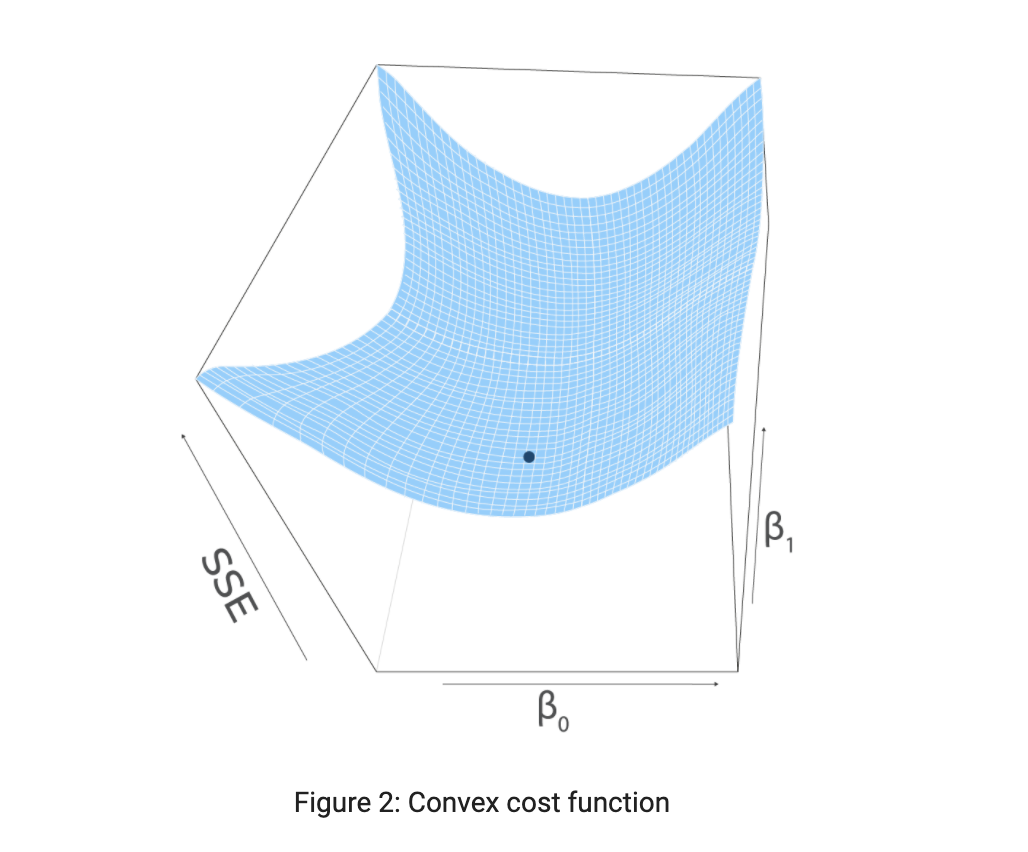
The parameters at a minimum point are obtained from calculus by setting the first derivative of the objective function to 0. Gradient or slope is always 0 at the minimum point. This statement is extended in the upcoming chapter, Gradient Descent in detail. We have two unknown parameters, intercept (𝛽0) and slope (𝛽1) so, we will take the partial derivative of SSE with respect to 𝛽0 and 𝛽1 separately. We will set both partial derivatives to 0 and solve for 𝛽0 and 𝛽1 separately.
Note: To avoid a little clutter in the derivation below, we will not include the summation index. As said earlier, the summation is always indexed from 1 to 𝑛, 𝑛 being the number of samples.
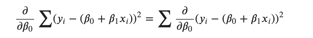
Taking partial derivatives with respect to 𝛽0:

Note that the derivative of the sum is the sum of the derivatives. So, we can take the derivative inside the summation.
Now, applying power rule and chain rule, we get:

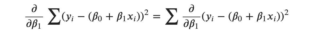
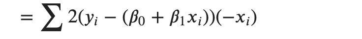
Now, with respect to 𝛽1:

Again, the derivative of the sum is the sum of the derivatives, So, we take the derivative inside the summation.
Applying power rule, 2 comes out front and exponent becomes 1 . We will also apply chain rule to encounter the coefficient of 𝛽1 .
Cleaning up a bit,

Now, we set up the partial derivatives equal to 0 for equation (1) and (2).

Here, we have two equations and two unknowns, and we are going to solve this to find our parameters. But how do we get that?
First, we will get an expression for 𝛽0 from the first equation. That expression would involve 𝛽1, and we will substitute that equation in the second equation and solve for 𝛽1. Let’s solve the first equation.
Solving for 𝛽0 equating equation (1) to 0,

We can divide both sides by −2 so that we get,

If we carry the summation term through each terms inside the bracket, we get:

Note that with respect to summation, 𝛽0 and 𝛽1 are constants. Statistically, they are random variables that take on any random value. But the values they take are constant over the samples. With respect to summation over the samples, they are constants so they can come outside the summation term as:

The sum of 𝛽0 from 1 to 𝑛 turns to 𝑛𝛽0 and 𝛽1 comes out of the summation term.
Now, isolating the 𝑛𝛽0 term, we get:

Dividing both sides by 𝑛, we get:

The sum of all 𝑦′𝑠 divided by 𝑛 gives the mean or average and so is for 𝑥′𝑠. So, we end up with:

But this doesn’t work without knowing the value of 𝛽1 . So, we substitute this expression of 𝛽0 to the equation where the partial derivative of 𝛽1 is set to 0.
Hence, solving for 𝛽1,
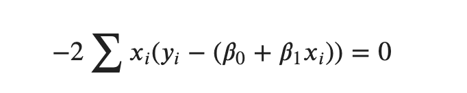
We can divide both sides by −2 so that we get,

Substituting 𝛽0, we get:

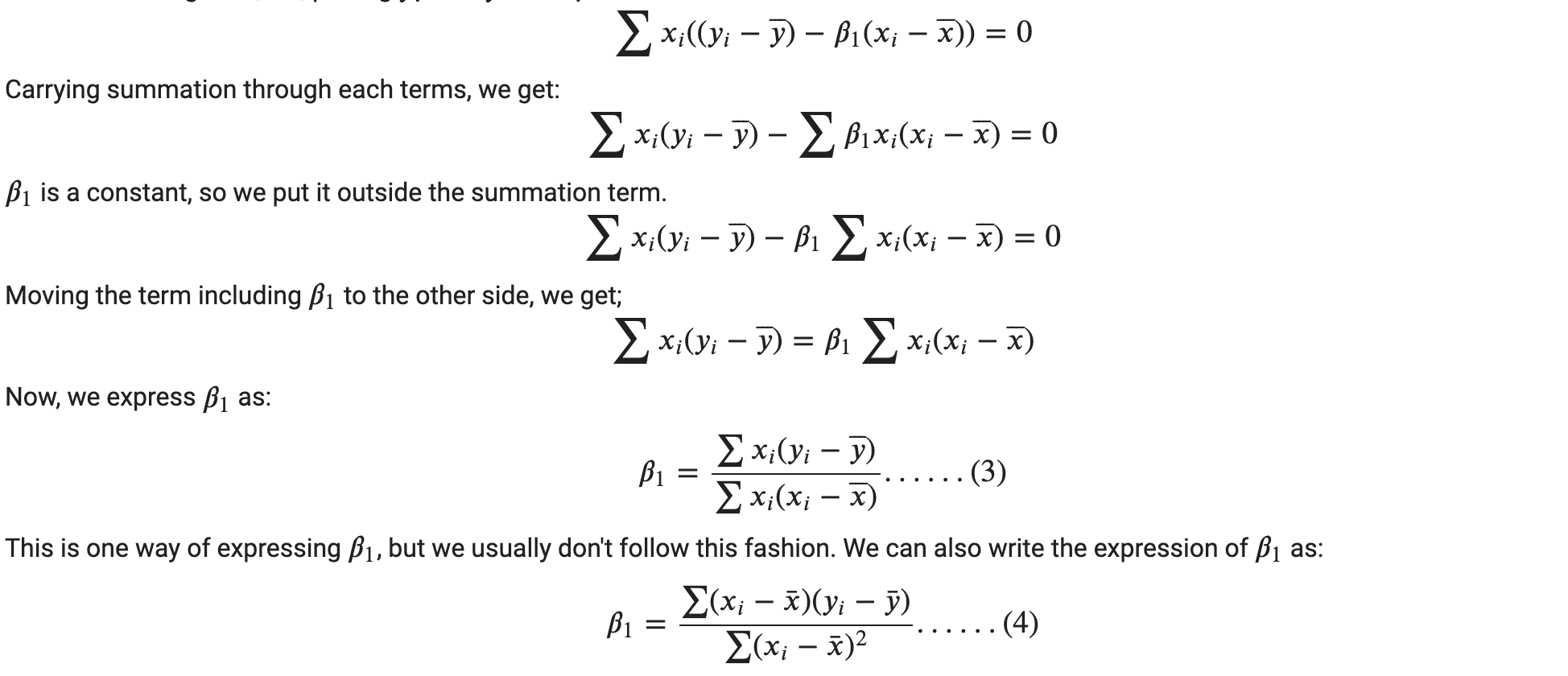
Now, we are getting somewhere since the unknown in the above expression is only 𝛽1 . Now, we will find a way to isolate 𝛽1 . Let’s first gather similar terms together.
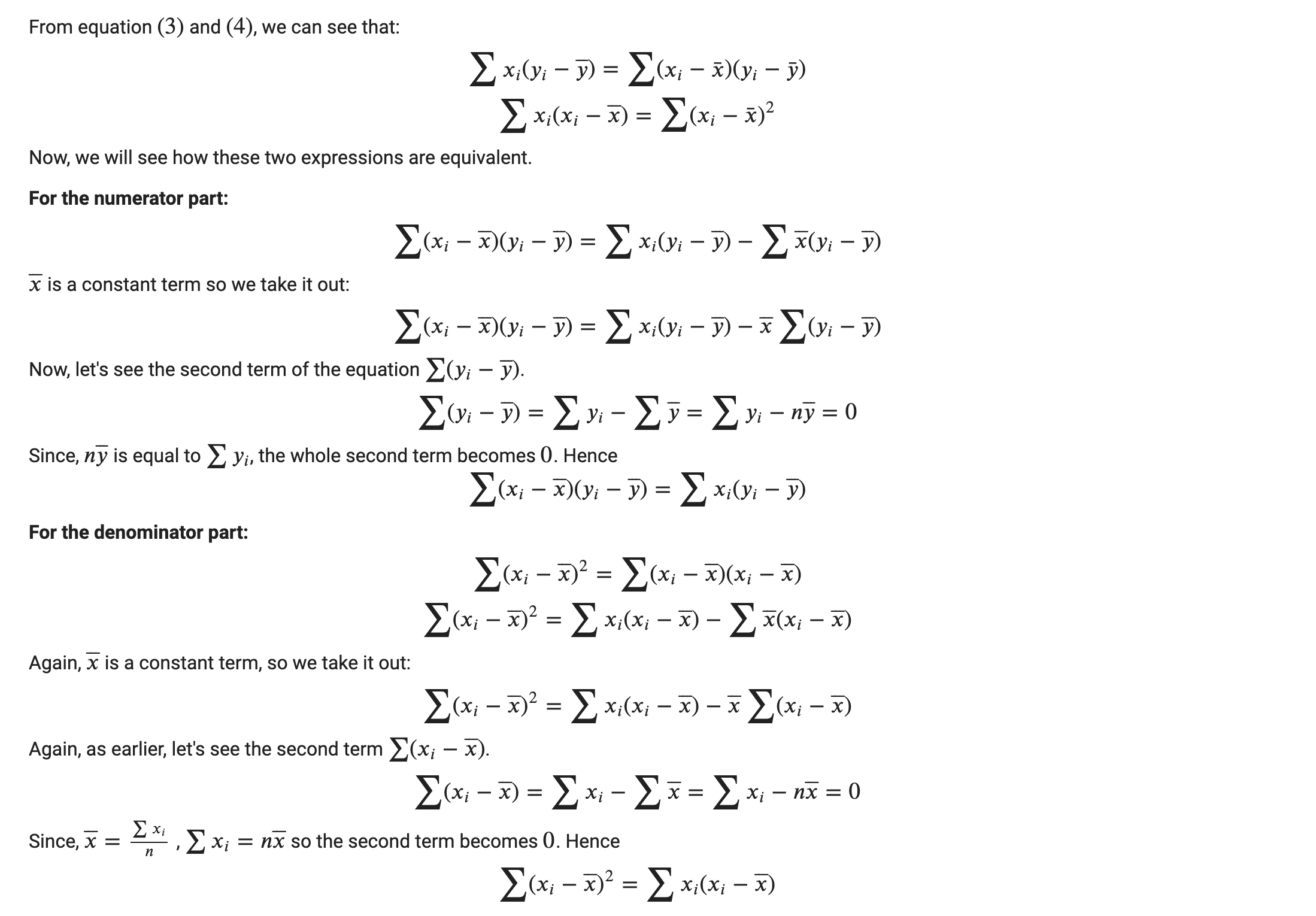
So, now we proved the similarity of the denominator and numerator terms of both expressions of 𝛽1 .
Since the parameters are estimates, we usually put hats on them. The key equations of the estimated parameters for simple linear regression are:

From the samples provided, first we find 𝛽1 from the first expression and substitute the value of 𝛽1 in the second expression for 𝛽0 .
Implementation on Real World Dataset For implementation, we will use same Advertising dataset.
A popular introductory statistics book, An Introduction to Statistical Learning, provides this dataset on their website. This dataset can be downloaded from the following address:
http://faculty.marshall.usc.edu/gareth-james/ISL/Advertising.csv This dataset has got three inputs as advertising mediums, i.e. TV, radio and newspaper. Similarly the output variable is sales. This is a sales prediction problem with investment in any of the advertising mediums.
# Imports
import numpy as np
import pandas as pd
import matplotlib as mpl
from matplotlib import pyplot as plt
data_path = "https://storage.googleapis.com/codehub-data/1-lv2-2-2-Advertisement.csv"

# Read the CSV data from the link
data_df = pd.read_csv(data_path,index_col=0)

# Print out first 5 samples from the DataFrame
data_df.head()
Output:
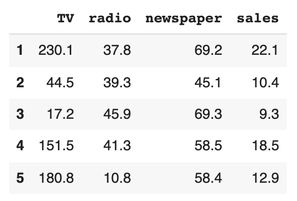
fig = plt.figure(figsize=(15,4))
gs = mpl.gridspec.GridSpec(1,3)

# Plot of sales vs TV
ax = fig.add_subplot(gs[0])
ax.scatter(data_df["TV"], data_df["sales"], color="red", marker=".")
ax.set_xlabel("TV")
ax.set_ylabel("sales")

# Plot of sales vs radio
ax = fig.add_subplot(gs[1])
ax.scatter(data_df["radio"], data_df["sales"], color="green", marker=".")
ax.set_xlabel("radio")
ax.set_ylabel("sales")

# Plot of sales vs newspaper
ax = fig.add_subplot(gs[2])
ax.scatter(data_df["newspaper"], data_df["sales"], color="blue", marker=".")
ax.set_xlabel("newspaper")
ax.set_ylabel("sales")

plt.show()
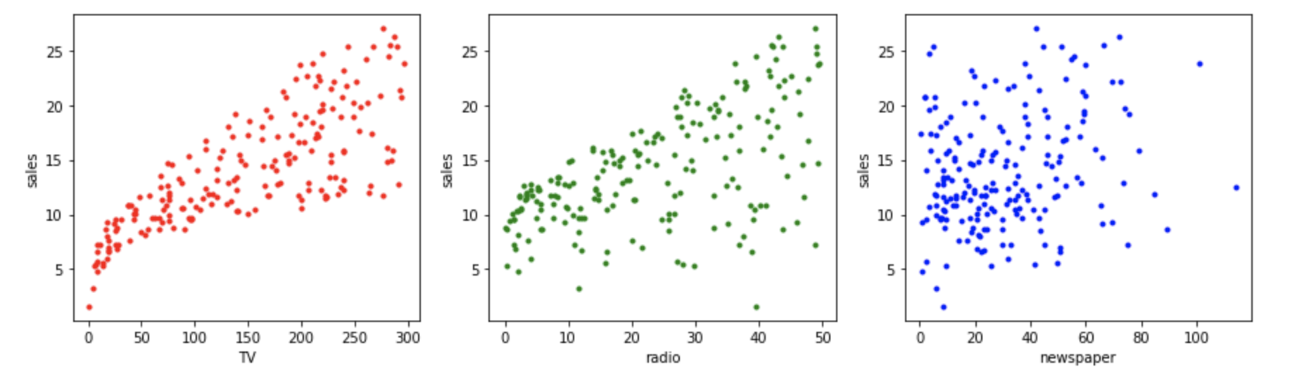
The first plot shows a sharp upward trend in the number of units sold as TV advertising increases. A similar trend is also found as radio advertising increases. However, in the last plot, there does not appear to be a relationship between newspaper advertising and the number of units sold.
Simple Linear Regression with Ordinary Least squares Earlier we used Scikit-Learn’s LinearRegression predictor object to estimate 𝛽0 and 𝛽1 . Now, we will implement the formulas derived from OLS to estimate the parameters.
fig = plt.figure(figsize=(15,4))
gs = mpl.gridspec.GridSpec(1,3)

# function for training model and plotting
def train_plot(data_df, feature, ax, c):

  # initializing our inputs and outputs
  X = data_df[[feature]].values
  Y = data_df[["sales"]].values

  # mean of our inputs and outputs
  x_mean = np.mean(X)
  y_mean = np.mean(Y)

  #total number of samples
  n = len(X)

  # using the OLS formula to calculate the b1 and b0
  numerator = 0
  denominator = 0
  for i in range(n):
    numerator += (X[i] - x_mean) * (Y[i] - y_mean)
    denominator += (X[i] - x_mean) ** 2

  b1 = numerator / denominator
  b0 = y_mean - (b1 * x_mean)
  y_hat = b0 + np.dot(X,b1)

  ##Plot the regression line
  ax.scatter(data_df[feature], data_df["sales"], color=c, marker=".")
  ax.plot(X, y_hat, color="black")
  ax.set_xlabel(feature)
  ax.set_ylabel("sales")
  ax.set_title(("$y$ = %3f + %3f$x$" %(b0, b1)))


# Train model using TV data to predict sales
ax0 = fig.add_subplot(gs[0])
train_plot(data_df, "TV", ax0, "red")

# Train model using radio data to predict sales
ax1 = fig.add_subplot(gs[1])
train_plot(data_df, "radio", ax1, "green")

# Train model using newspaper data to predict sales
ax2 = fig.add_subplot(gs[2])
train_plot(data_df, "newspaper", ax2, "blue")

plt.show()
Here, we performed a simple linear regression in each of the scatter plots.
TV vs. sales
TV is the input variable, one of the advertising mediums and sales is the output variable. Parameters estimated from OLS has done pretty good work in fitting the data points. The intercept ( 𝛽0 ) has been estimated as 7.03 and slope ( 𝛽1 ) has been estimated as 0.04 . The values of the parameters through OLS are the same to that through Scikit-Learn. The first plot depicts the simple linear regression with input as TV and output as sales.
radio vs. sales
radio is the input variable, one of the advertising mediums, and sales is the output variable. Parameters estimated from OLS has done pretty good work in fitting the data points. The intercept ( 𝛽0 ) has been estimated as 9.31 and slope ( 𝛽1 ) has been estimated as 0.21 . The values of the parameters through OLS are the same to that through Scikit-Learn.The second plot depicts the simple linear regression with input as radio and output as sales.
newspaper vs. sales
newspaper is the input variable, which is one of the advertising mediums, and sales is the output variable. Parameters estimated from OLS has done pretty good work in fitting the data points. The intercept ( 𝛽0 ) has been estimated as 12.35 and slope ( 𝛽1 ) has been estimated as 0.05 . The values of the parameters through OLS is the same as that through Scikit-Learn.The third plot depicts the simple linear regression with input as newspaper and output as sales.
You can check out previous reading material to ensure the similarity of the values of parameters.
Comments