Understanding Linear Regression [3/3]

2 minute read

Now that you have estimated the parameters for simple linear regression with OLS let’s do the same for multiple linear regression.

From L1 content, you have the idea of Multiple Linear Regression. Let’s recall a bit. Multiple linear regression generalizes simple linear regression by allowing more than one input variable: 𝑥1,𝑥2,…,𝑥𝑑 . The goal of multiple linear regression is to find a relationship between the input variables and the output variable. This relationship is represented mathematically as follows:

𝛽1 through 𝛽𝑑 are the estimated regression coefficients for the independent variables 𝑥1 through 𝑥𝑑 . As in simple linear regression, the regression model to get actual output variable is:

𝜖 is the random error or residual, which reflects the difference between the actual output point and predicted output point.

Multiple linear regression involves more than one input variable, so it is impossible to individually derive a solution for each regression coefficient for each input variable. In a sophisticated regression problem dimension (𝑑 ) can range to very higher values.

So, how do we estimate all regression coefficients?

From multiple linear regresssion model, we have:

We have 𝑛 set of observations. So we can write:

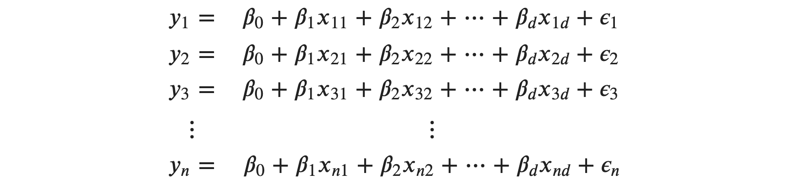
Xnd is the 𝑛th observation for 𝑑th feature or input variable. These 𝑛 set of equations can be written in matrix form as:

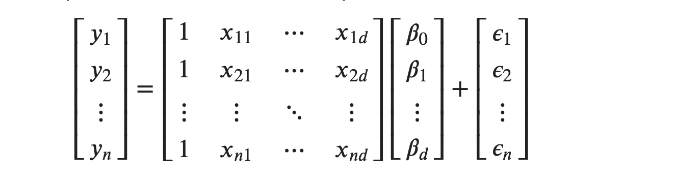
Using mathematical notations, we can write as:

𝐲 is a n×1 column matrix where each element is the observed value of output variable. Similarly, 𝐗 is n×(d+1) matrix. An extra dimension is due to the inclusion of 1′𝑠 in the first column. You can interpret the first column, including 1′s as being multiplied against 𝛽0. There are (d+1) unknown parameters, d regression coefficients for each of the input variables and 1 extra for the intercept, 𝛽0 .So 𝜷 is (d+1)×1 column matrix.

By now, we addressed the multiple features and multiple unknown parameters properly in the form of a matrix. Now, we roll back to the principle of OLS to determine the unknown parameters.

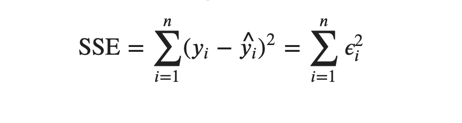
From OLS, our objective is to find a column matrix or a column vector, 𝜷, such that Sum of Squared Errors, SSE is minimum. SSE is written as:

Since

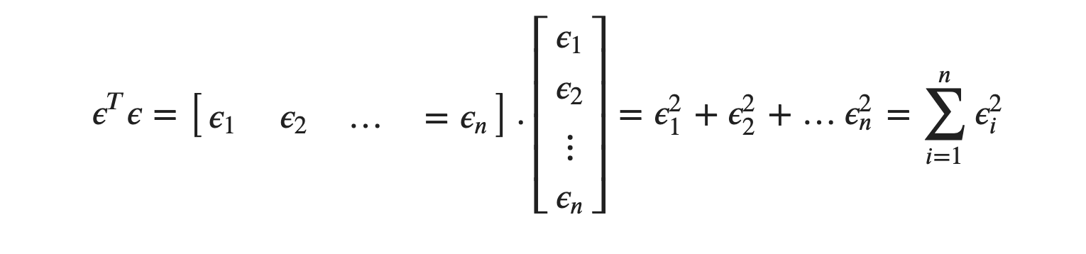
We can also write SSE as:

From equation (1), we know that

so we can also write SSE as:

This positive quadratic error function or SSE or objective function is always a convex surface facing upwards as in a simple linear equation. From calculus, the value of parameters at the minimum point is obtained by setting the first derivative of the objective function, with respect to the parameters, equal to 0. So, we will take the partial derivative of the objective function, with respect to 𝜷, and get the value for the column matrix, 𝜷.

You can take a pen and paper and try expanding the product term to the sums. You have to use basic transpose rules and matrix multiplication rules. That’s it! Now, we will set the derivative to 0 as: